
The Hidden Economics of LLM Inference
In AI, conversations often center around new architectures, reinforcement learning breakthroughs, and ever-larger open-source releases. This leaves remarkably little attention to what happens after training, when you actually need to serve that model to users at production scale.
At Hebbia, we think the focus imbalance on model training over running inference deserves more scrutiny in order to build economical AI solutions. We recently ran an internal research project to stress-test two questions:
- Can a fine-tuned open-source model match frontier-model quality?
- Can we actually serve the model cost-effectively?
The answers to these questions were asymmetric. To achieve balance, our research team pursued developing capacity planning frameworks to make informed decisions about how to serve the best possible model for our tasks while maintaining low latencies and costs.
Through this work we are bringing a new perspective to the build versus buy question in the AI industry.
Why Long-Context Inference Is So Expensive
We fine-tuned multiple Qwen3-14 & 32B models for high fidelity span extraction and achieved extraction quality on par with current SOTA frontier models as well as an 8–9 point improvement in exactness and correctness. All this with a ~43x reduction in parameter size.
When we distilled capability into a smaller model (14B–32B parameters), our 32B model in FP8 needed ~32GB of weights, leaving ample headroom on an 80GB H100 for KV-cache at 80k context. We consistently saw KV-cache memory utilization at only 20–30%, while GPU volatile utilization reported 80–85% under single-request load. At first glance, this looks purely compute-bound.
But GPU volatile utilization is a blunt instrument. It doesn't distinguish between cycles spent on tensor core math and cycles stalled waiting on memory reads. In practice, the two bottlenecks layer on top of each other depending on the inference phase:
- Prefill (processing all input tokens in parallel): the large matrix multiplications in attention and FFN layers keep the tensor cores busy.
- Decode (generating output tokens one at a time): each step must read the full KV cache for every attention layer, and with 80k tokens of context, tens of gigabytes per step move through HBM
A single request may sit comfortably under the H100's ~3.35 TB/s bandwidth ceiling, but the operation is fundamentally bandwidth-bound. This prefill-compute/decode-bandwidth split is well-established: FlashAttention was designed around the insight that HBM access dominates attention cost, the vLLM project's roofline analysis treats it as the foundational design constraint, and recent empirical work confirms that even large-batch decode remains memory-bound with most GPU compute underutilized.
Figure 1: Prefill processes all input tokens in one parallel forward pass (2–4s). Generation produces output tokens sequentially: m forward passes for m tokens (10–15s). The sequential phase dominates total latency.
Why Batching Is Not the Solution
In standard LLM serving, continuous batching amortizes GPU cost across requests by processing multiple requests simultaneously. For short-context workloads where the KV cache is small, there is ample HBM bandwidth headroom to serve additional requests in parallel, yielding 4–8x throughput gains.
For our long-context workload, a single 80k-context decode already pushes close to the HBM bandwidth ceiling, leaving almost no headroom to share. When you try to batch multiple such requests, you multiply the KV traffic competing for the same bandwidth, increase cache miss and paging overhead (if using paged KV allocation), and lose kernel efficiency as memory access patterns become less predictable. The result is heavy contention. Each additional request makes every other request slower.
Our benchmarks confirmed this directly. Moving from 1 to 3 concurrent requests actually inflated end-to-end latency by 13–40x across model sizes. A third-party inference provider reproduced this behavior independently using both vLLM and SGLang, ruling out configuration artifacts.
In plain terms: Your cost is no longer driven by throughput efficiency. It's driven entirely by demand volatility.
The Queueing Theory Solution
When a telephone exchange receives calls faster than operators can answer, calls queue. Too few operators and callers hang up; too many and operators sit idle.
Compute allocation experiences this same challenge. If each GPU serves only one request at a time, fleet sizing becomes a classical queueing problem: how many servers do you need to handle stochastic arrivals without violating latency SLOs?
The Erlang-C model (M/M/c queue) provides closed-form solutions for sizing the operator pool (or in our case, the GPU fleet) given arrival rates, service times, and target wait-time guarantees.
GPU Inference Reality | Erlang-C Assumption |
|---|---|
User requests arrive stochastically | Poisson arrivals |
Latency varies with input/output length | Exponential service times |
Homogeneous GPU fleet | c identical servers |
Load balancer distributing to available GPUs | Single FIFO queue |
The Erlang-C Formula
The key quantity is offered load per server: ρ = λ / (c × μ) = (λ × S) / c, where λ is arrival rate, S is mean service time, c is GPU count, and ρ is utilization. For stability, ρ must be < 1.
C(c, λ/μ) = [1 + (1-ρ) × (c! / (λ/μ)^c) × Σ(k=0 to c-1) (λ/μ)^k / k!]^(-1)
E[Wq] = C(c, λ/μ) × S / (c × (1 - ρ))
The (1 - ρ) denominator is the critical insight: small increases in utilization produce enormous increases in wait time.
In practice, this nonlinearity looks like:
Utilization (ρ) | Wait Time Multiplier |
|---|---|
50% | 2× baseline |
80% | 5× baseline |
90% | 10× baseline |
95% | 20× baseline |
Running GPU fleets at high utilization while maintaining latency SLOs is not only an operational constraint, it’s also a mathematical one.
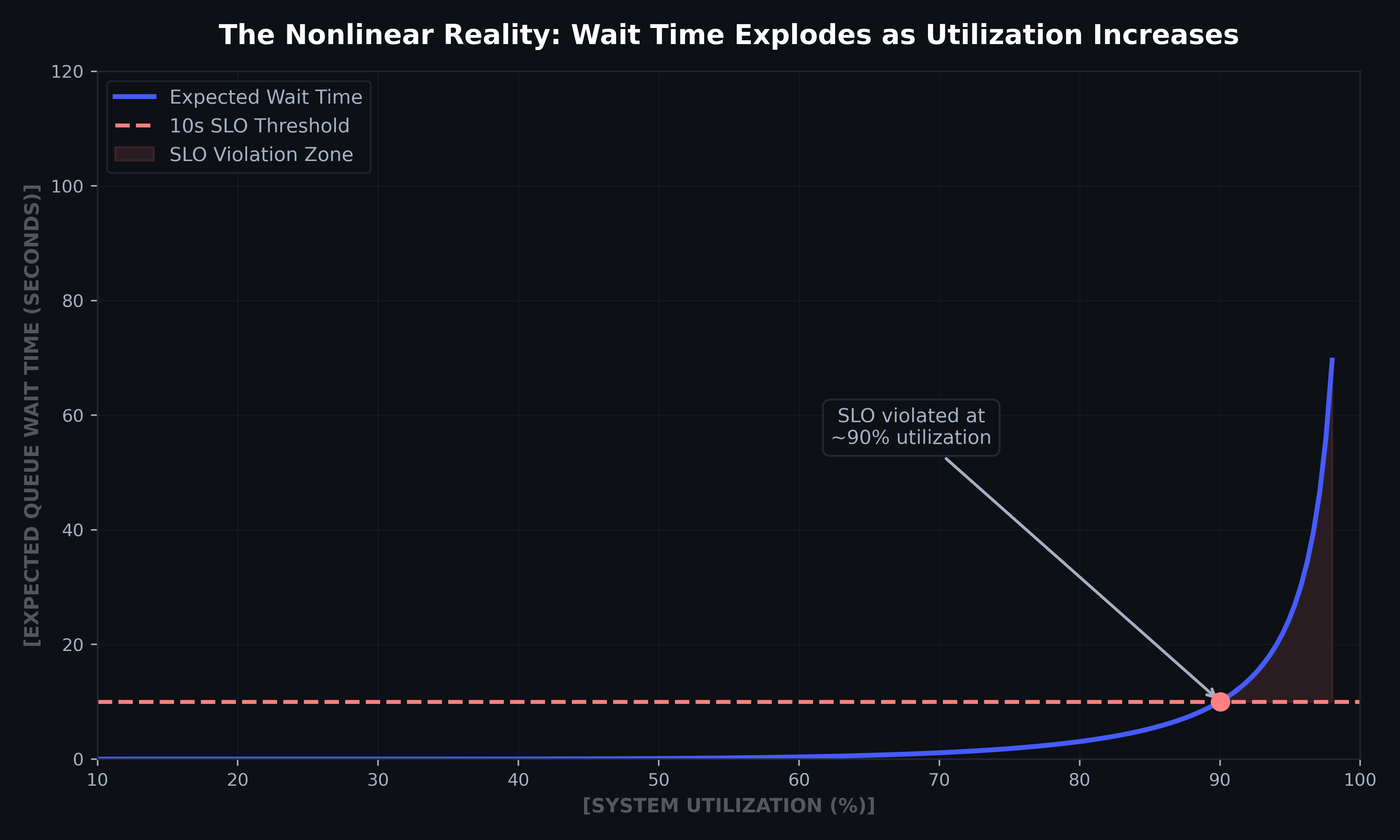
Figure 2: Expected queue wait time vs. system utilization for a 10-GPU fleet. The curve stays near zero through moderate utilization, then rises sharply. By ~90% utilization, queue wait crosses the 10s SLO threshold and continues climbing steeply. Computed via Erlang-C with S=15s, c=10 GPUs.
Erlang-C Applied
A worked example shows how fast this bites:
- Mean service time per request S = 15 seconds
- Demand spikes to λ = 100 req/min
- c = 10 GPUs
- Queue grows unbounded ρ = 2.5
GPU fleets must be sized for peak demand, not average, requiring 31 GPUs to bring utilization down to 0.8. Here we’ve highlighted the crux of the problem: demand volatility.
Real enterprise demand isn't steady-state. It spikes around filing deadlines, deal workflows, and market events. Consider two workloads with identical average volume:
- Workload A (Smooth): 50 req/min constant → ~16 GPUs needed
- Workload B (Bursty): 10 req/min baseline with 400 req/min spikes → ~125 GPUs needed
Highly volatile demand requires 8× more capacity for the same average volume. You pay for 125 GPUs 90% of the time when only 3–4 are active, leaving 97% of your GPUs idle.
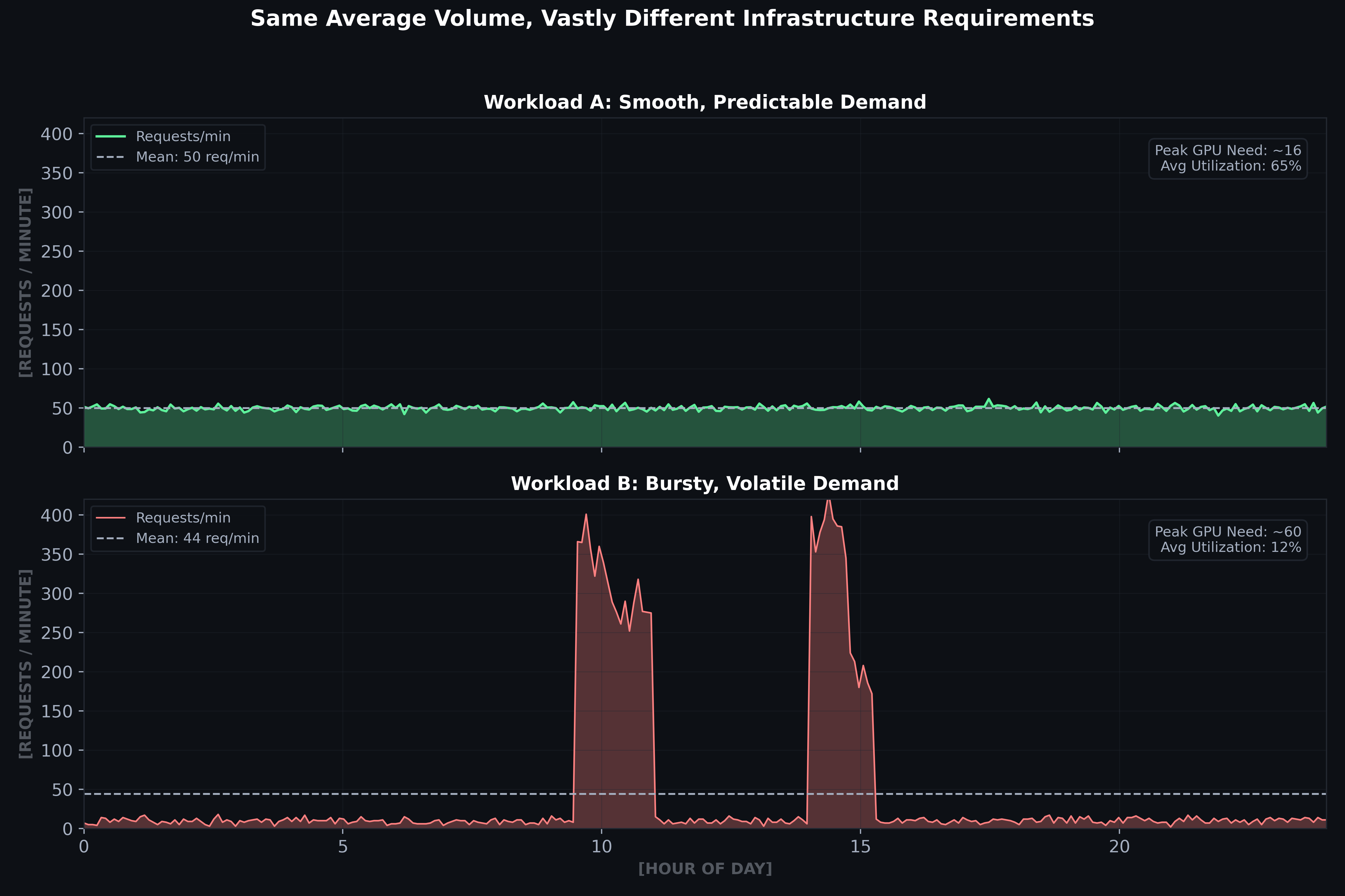
Figure 3: Same average volume, vastly different capacity requirements. Bursty demand forces provisioning for peaks, with only ~12% average utilization. Erlang-C capacity computed with S=15s, target ρ<0.8.
Autoscaling helps but can't fully compensate, as demand spikes arrive faster than GPU cold starts. Further, autoscaling introduces hysteresis: capacity lags as demand increases (warmup delay) and decreases (graceful cooldown to avoid flapping). The result is persistent over-provisioning or under-provisioning, often both in the same hour.
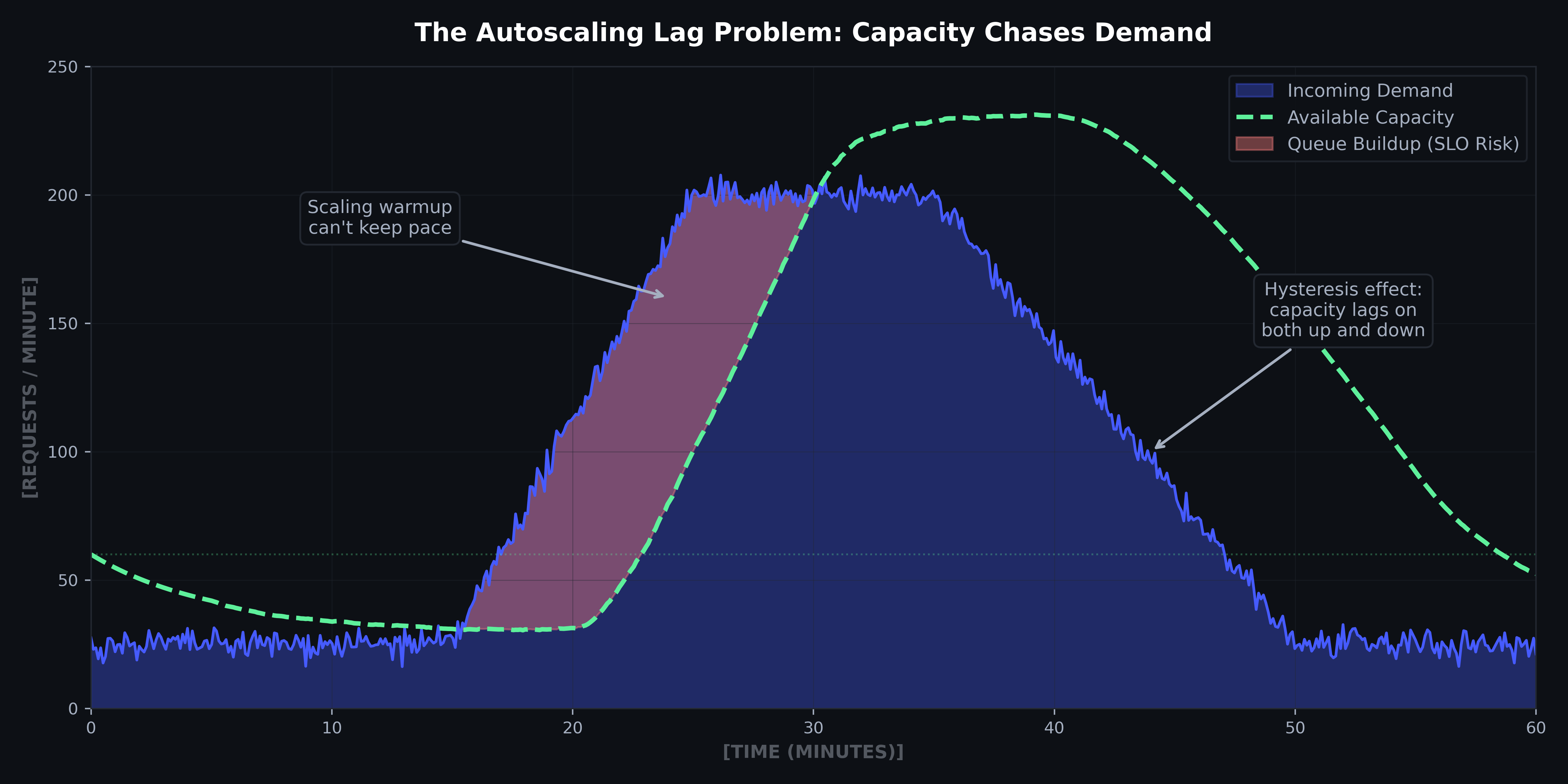
Figure 4: Autoscaling lag causes queue buildup during rapid demand ramps. Capacity also lags on scale-down due to hysteresis, creating idle cost. 60-minute simulation with 5-minute warmup lag.
Why API Providers Win on Economics
Systems engineering is what competitive inference looks like today. As context windows expand and architectures become more specialized, the operational complexity of running your own fleet increases.
The queueing analysis above explains why API providers’ ability to aggregate demand has structural cost advantages that go beyond model quality or operational expertise. If n customers each have independent demand with variance σ², the pooled coefficient of variation (CV) decreases as 1/√n. A provider serving 1,000 customers sees 1/30th the relative standard deviation of any individual customer.
Meeting enterprise demand has a spectrum of pooling:
- Frontier Model API providers (OpenAI, Anthropic, Google) pool demand across all customers worldwide. Your 2pm spike coincides with another customer's lull. Under the law of large numbers, the aggregate demand curve is dramatically smoother than any individual customer's.
- Third-party inference platforms (Baseten, Modal, Fireworks) pool demand across all customers running open-weight models. They've solved the queueing problem with warm GPU pools, speculative decoding, and fixed costs spread across tenants.
- Self-hosting removes the advantage of a smoothed demand curve, forcing providers to absorb variance in full.
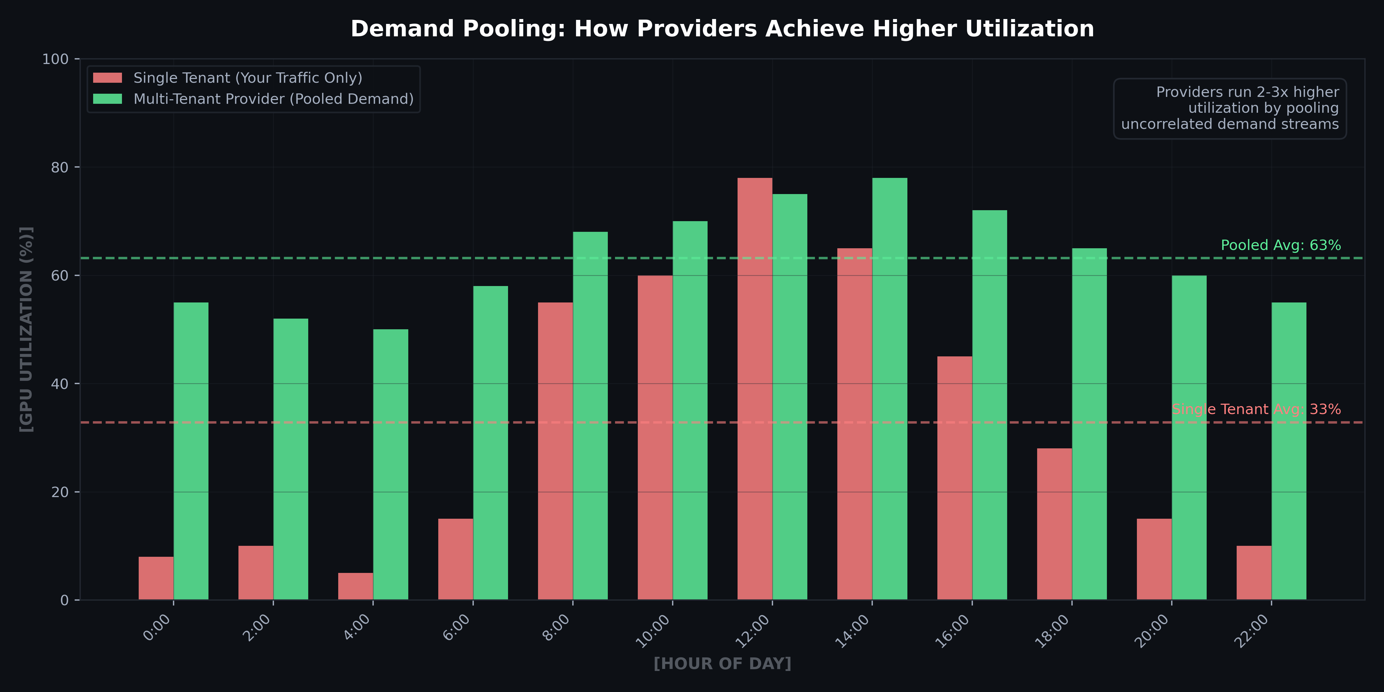
Figure 5: Multi-tenant providers achieve 2–3× higher GPU utilization than single-tenant operation by pooling uncorrelated demand streams across customers and time zones. Illustrative hourly utilization comparison.
Third-party inference providers offer a middle path for teams that need a specific open-weight or fine-tuned model but don't want to build GPU fleet management from scratch. Though you are left to inherit the platform's latency characteristics (cold-start behavior and pricing model), for many teams it is worth the tradeoff. API pricing is invariant to your variance; the provider absorbs it across their customer base. The crossover occurs at CV ≈ 0.3–0.5 depending on SLO targets and autoscaling capabilities.
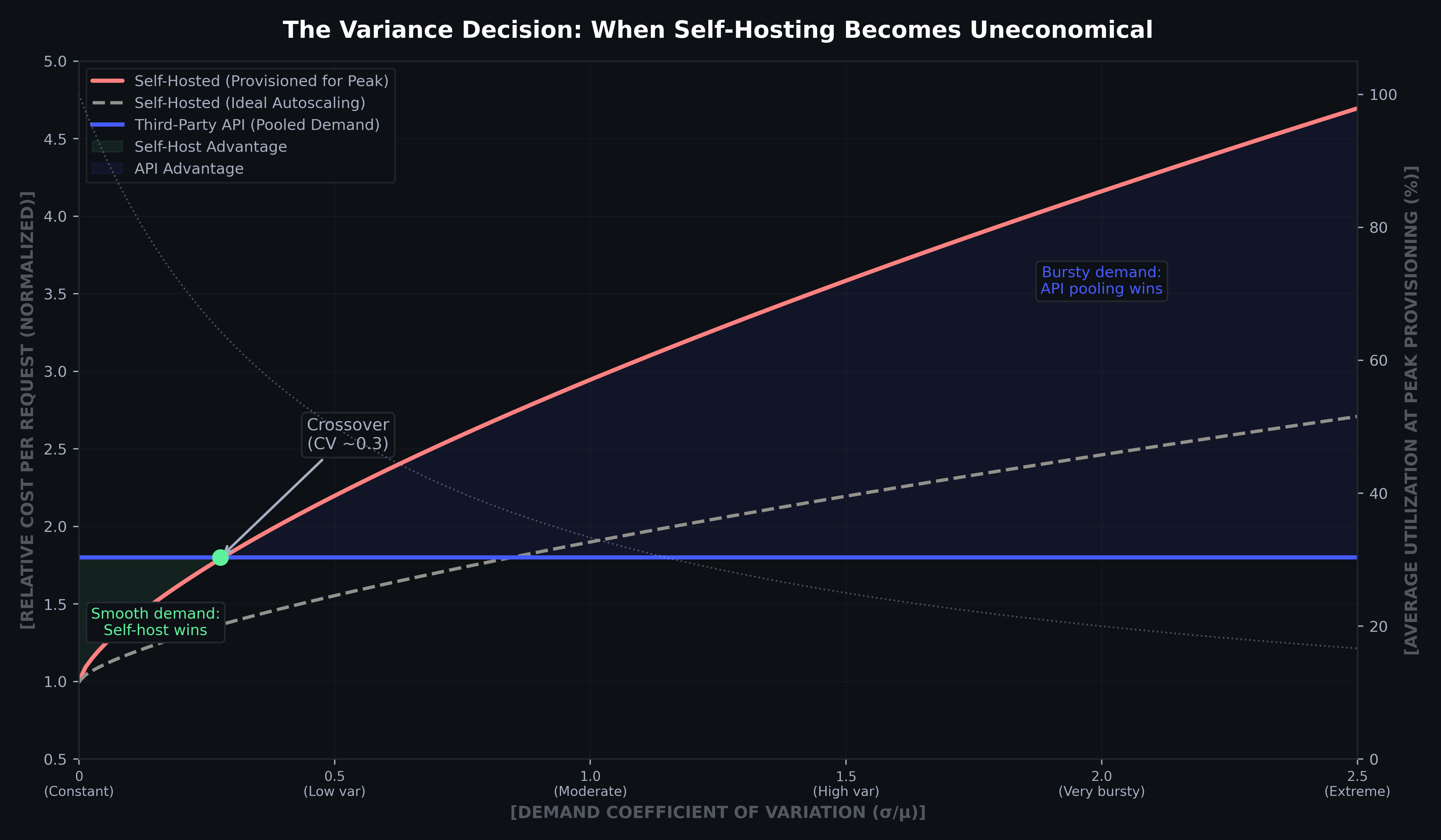
Figure 6: Cost vs. demand coefficient of variation (CV = σ/μ). As modeled self-hosting is economical only at CV < 0.3–0.4. At higher variance, API demand pooling is structurally cheaper. The secondary axis (dotted) shows how utilization collapses as variance rises. Cost curves normalized to API baseline.
Conclusion
We set out to determine whether a fine-tuned open-source model could replace frontier APIs for evidence extraction by answering 2 questions:
- Can a fine-tuned open-source model match frontier-model quality?
Yes, distillation and targeted fine tuning works.
- Can we actually serve the model cost-effectively?
The answer is more complex. On economics, current hardware constraints make self-hosting unviable for many workload profiles.
Our findings don’t mean that self-hosting never works, however. For workloads with smooth, predictable demand and short service times (prefill heavy vs decode heavy), it can be the right choice. The reality is though that the vast majority of enterprise AI workloads don’t meet these conditions, making self-hosting impractical.
The hidden advantage of third-party providers, whether frontier APIs or inference platforms, is that they've already solved the queueing, scaling, and utilization problems that any self-hosted deployment will inevitably face.
The generalizable lesson: before you invest in training, make sure you can afford to serve. For self-hosted LLM inference, demand variance, not volume, drives the economics. The Erlang-C model shows exactly how cost scales with the gap between peak and average load. But we know economics isn't the only variable. Data sovereignty, regulatory constraints, model control, and strategic considerations all factor in. The right answer depends on your situation.
Further Reading
- Dao et al., FlashAttention: Fast and Memory-Efficient Exact Attention with IO-Awareness (NeurIPS 2022) – the foundational work on IO-aware attention, showing that minimizing HBM data movement is the key to fast transformer inference.
- Recasens et al., Mind the Memory Gap: Unveiling GPU Bottlenecks in Large-Batch LLM Inference (IEEE CLOUD 2025) – empirical evidence that large-batch decode remains memory-bound, with GPU compute underutilized due to DRAM bandwidth saturation.
- Yuan et al., LLM Inference Unveiled: Survey and Roofline Model Insights (2024) – comprehensive survey analyzing inference bottlenecks through the roofline model, with an open-source analysis tool (LLM-Viewer).
- Inside vLLM: How LLM Inference Works Under the Hood (2025) – deep architectural walkthrough of continuous batching, paged attention, speculative decoding, and the prefill/decode roofline model.
- Optimizing Inference for Long Context with NVFP4 KV Cache (NVIDIA, 2025) – 4-bit KV-cache quantization achieving 50% memory reduction and doubled batch capacity at <1% accuracy cost.
- Extreme Hardware-Software Co-Design for Sarvam AI (NVIDIA, 2025) – production case study: fused kernels, disaggregated serving, mixed scheduling, and NVFP4 on Blackwell for a 4x throughput gain.


